
AA228V/CS238V
Validation of Safety-Critical Systems
Validation of Safety-Critical Systems
Lecture 09: Failure Distribution
Sydney Katz (smkatz@stanford.edu)
Sydney Katz (smkatz@stanford.edu)
What is the failure distribution?
Trajectory Distribution
p(τ)
Trajectory Distribution
p(τ)
Failure Distribution
p(τ∣τ∈/ψ)
p(τ∣τ∈/ψ)=
1{τ∈/ψ}p(τ)
∫1{τ∈/ψ}p(τ)dτ
p(τ∣τ∈/ψ)=
1{τ∈/ψ}p(τ)
∫1{τ∈/ψ}p(τ)dτ
p(τ∣τ∈/ψ)=
1{τ∈/ψ}p(τ)
∫1{τ∈/ψ}p(τ)dτ
A Simple Example
p(τ∣τ∈/ψ)=
1{τ∈/ψ}p(τ)
∫1{τ∈/ψ}p(τ)dτ
p(τ∣τ∈/ψ)=
1{τ∈/ψ}p(τ)
∫1{τ∈/ψ}p(τ)dτ
A Simple Example
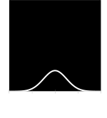
p(τ)
τ∈/ψ
τ∈ψ
p(τ∣τ∈/ψ)=
1{τ∈/ψ}p(τ)
∫1{τ∈/ψ}p(τ)dτ
p(τ∣τ∈/ψ)=
1{τ∈/ψ}p(τ)
∫1{τ∈/ψ}p(τ)dτ
A Simple Example
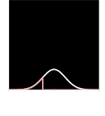
p(τ)
1{τ∈/ψ}p(τ)
p(τ∣τ∈/ψ)=
1{τ∈/ψ}p(τ)
∫1{τ∈/ψ}p(τ)dτ
p(τ∣τ∈/ψ)=
1{τ∈/ψ}p(τ)
∫1{τ∈/ψ}p(τ)dτ
A Simple Example
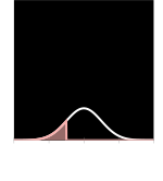
p(τ)
1{τ∈/ψ}p(τ)
∫1{τ∈/ψ}p(τ)dτ
p(τ∣τ∈/ψ)=
1{τ∈/ψ}p(τ)
∫1{τ∈/ψ}p(τ)dτ
A Simple Example
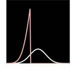
p(τ∣τ∈/ψ)
gives us the shape
p(τ∣τ∈/ψ)=
1{τ∈/ψ}p(τ)
∫1{τ∈/ψ}p(τ)dτ
A Simple Example
p(τ∣τ∈/ψ)
gives us the normalizing
constant
constant
p(τ∣τ∈/ψ)=
1{τ∈/ψ}p(τ)
∫1{τ∈/ψ}p(τ)dτ
normally, this normalizing
constant is very difficult if not
impossible to compute
constant is very difficult if not
impossible to compute
p(τ∣τ∈/ψ)=
1{τ∈/ψ}p(τ)
∫1{τ∈/ψ}p(τ)dτ
We can compute this!
Unnormalized Probability Density
1{τ∈/ψ}p(τ)
Unnormalized Probability Density
pˉ(τ∣τ∈/ψ)=
1{τ∈/ψ}p(τ)

There are algorithms that allow us to
draw samples from an unnormalized
probability density! This way, we can
implicitly represent the failure
distribution using samples.
draw samples from an unnormalized
probability density! This way, we can
implicitly represent the failure
distribution using samples.
Unnormalized Probability Density
pˉ(τ∣τ∈/ψ)=
1{τ∈/ψ}p(τ)
There are algorithms that allow us to
draw samples from an unnormalized
probability density! This way, we can
implicitly represent the failure
distribution using samples.
draw samples from an unnormalized
probability density! This way, we can
implicitly represent the failure
distribution using samples.
Plan for Today
1
Unnormalized Probability Density
2
Rejection Sampling
3
Markov Chain Monte Carlo
4
Tips to Scale Things Up
Rejection Sampling
Rejection Sampling
Dart Board Analogy
0.6
0
−3
3
τ
h
0.6
0
−3
3
τ
h
1
Throw darts uniformly at the board.
a
Sample a value uniformly between −3 and 3
0.6
0
−3
3
τ
h
1
Throw darts uniformly at the board.
a
Sample a value uniformly between −3 and 3
b
Sample a value uniformly between 0 and 0.6
repeat for
each dart
each dart
0.6
0
−3
3
τ
h
1
Throw darts uniformly at the board.
a
Sample a value uniformly between −3 and 3
b
Sample a value uniformly between 0 and 0.6
repeat for
each dart
each dart
0.6
0
−3
3
τ
h
1
Throw darts uniformly at the board.
a
Sample a value uniformly between −3 and 3
b
Sample a value uniformly between 0 and 0.6
repeat for
each dart
each dart
2
Reject any darts that lie
above the blue density.
above the blue density.
0.6
0
−3
3
τ
h
1
Throw darts uniformly at the board.
a
Sample a value uniformly between −3 and 3
b
Sample a value uniformly between 0 and 0.6
repeat for
each dart
each dart
2
Reject any darts that lie
above the blue density.
above the blue density.
3
Move the remaining darts to
the bottom of the board.
the bottom of the board.
0.6
0
−3
3
τ
h
pˉ(τ)
1
Throw darts uniformly at the board.
a
Sample a value uniformly between −3 and 3
τ∼q(⋅), q(τ)=U(−3,3)
b
Sample a value uniformly between 0 and 0.6
repeat for
each dart
each dart
2
Reject any darts that lie
above the blue density.
above the blue density.
3
Move the remaining darts to
the bottom of the board.
the bottom of the board.
q(τ)
0.6
0
−3
3
τ
h
pˉ(τ)
1
Throw darts uniformly at the board.
a
Sample a value uniformly between −3 and 3
τ∼q(⋅), q(τ)=U(−3,3)
b
Sample a value uniformly between 0 and 0.6
h=(cq(τ))(r), r∼U(0,1)
repeat for
each dart
each dart
2
Reject any darts that lie
above the blue density.
above the blue density.
3
Move the remaining darts to
the bottom of the board.
the bottom of the board.
q(τ)
0.6
0
−3
3
τ
h
pˉ(τ)
1
Throw darts uniformly at the board.
a
Sample a value uniformly between −3 and 3
τ∼q(⋅), q(τ)=U(−3,3)
b
Sample a value uniformly between 0 and 0.6
h=(cq(τ))(r), r∼U(0,1)
repeat for
each dart
each dart
2
Reject any darts that lie
above the blue density.
above the blue density.
3
Move the remaining darts to
the bottom of the board.
the bottom of the board.
q(τ)
c
0.6
0
−3
3
τ
h
pˉ(τ)
1
Throw darts uniformly at the board.
a
Sample a value uniformly between −3 and 3
τ∼q(⋅), q(τ)=U(−3,3)
b
Sample a value uniformly between 0 and 0.6
h=(cq(τ))(r), r∼U(0,1)
repeat for
each dart
each dart
2
Reject any darts that lie
above the blue density.
above the blue density.
Reject if (cq(τ))(r) > pˉ(τ)
3
Move the remaining darts to
the bottom of the board.
the bottom of the board.
q(τ)
c
0.6
0
−3
3
τ
h
pˉ(τ)
1
Throw darts uniformly at the board.
a
Sample a value uniformly between −3 and 3
τ∼q(⋅), q(τ)=U(−3,3)
b
Sample a value uniformly between 0 and 0.6
h=(cq(τ))(r), r∼U(0,1)
repeat for
each dart
each dart
2
Reject any darts that lie
above the blue density.
above the blue density.
Reject if (cq(τ))(r) > pˉ(τ)
3
Move the remaining darts to
the bottom of the board.
the bottom of the board.
Just keep the τ value for each sample
q(τ)
c
0.6
0
−3
3
τ
h
pˉ(τ)
1
Throw darts uniformly at the board.
a
Sample a value uniformly between −3 and 3
τ∼q(⋅), q(τ)=U(−3,3)
b
Sample a value uniformly between 0 and 1
h=(cq(τ))(r), r∼U(0,1)
repeat for
each dart
each dart
2
Reject any darts that lie
above the blue density.
above the blue density.
Reject if (cq(τ))(r) > pˉ(τ)
3
Move the remaining darts to
the bottom of the board.
the bottom of the board.
Just keep the τ value for each sample
q(τ)
c
Look at all those gray darts (samples) we wasted!
0
−3
3
τ
pˉ(τ)
1
Throw darts uniformly at the board.
a
Sample a value uniformly between −3 and 3
τ∼q(⋅), q(τ)=U(−3,3)
b
Sample a value uniformly between 0 and 0.6
h=(cq(τ))(r), r∼U(0,1)
repeat for
each dart
each dart
2
Reject any darts that lie
above the blue density.
above the blue density.
Reject if (cq(τ))(r) > pˉ(τ)
3
Move the remaining darts to
the bottom of the board.
the bottom of the board.
Just keep the τ value for each sample
q(τ)
c
Look at all those gray darts (samples) we wasted!
What if we could make our dart board look like this instead?
0
−3
3
τ
pˉ(τ)
1
Throw darts uniformly at the board.
a
Sample a value uniformly between −3 and 3
τ∼q(⋅), q(τ)=U(−3,3)
b
Sample a value uniformly between 0 and 0.6
h=(cq(τ))(r), r∼U(0,1)
repeat for
each dart
each dart
2
Reject any darts that lie
above the blue density.
above the blue density.
Reject if (cq(τ))(r) > pˉ(τ)
3
Move the remaining darts to
the bottom of the board.
the bottom of the board.
Just keep the τ value for each sample
q(τ)
c
What if we could make our dart board look like this instead?
We just need to select q(τ) to be a distribution we can sample from
and c such that cq(τ) is always greater than pˉ(τ).
and c such that cq(τ) is always greater than pˉ(τ).
Departing from the dart board analogy.

Departing from the dart board analogy.
But first, a random fact about darts:

Dart boards are designed to
reward accuracy and penalize
inaccuracy.
reward accuracy and penalize
inaccuracy.
Rejection Sampling
1
Sample τ∼q(⋅)
q(τ) is often referred to as a proposal distribution
2
Reject if cq(τ)r>pˉ(τ)
Rejection Sampling
1
Sample τ∼q(⋅)
q(τ) is often referred to as a proposal distribution
2
Reject if cq(τ)r>pˉ(τ)
r>
pˉ(τ)cq(τ)
Rejection Sampling
1
Sample τ∼q(⋅)
q(τ) is often referred to as a proposal distribution
2
Reject if cq(τ)r>pˉ(τ)
r>
pˉ(τ)cq(τ)
Accept if
r<
pˉ(τ)cq(τ)
rand()
Note: we must select the proposal
distribution q(τ) such that pˉ(τ)≤cq(τ).
distribution q(τ) such that pˉ(τ)≤cq(τ).
Rejection Sampling
Back to trying to sample from the failure distribution:
1
Sample τ∼q(⋅)
2
Accept if
r<
pˉ(τ)cq(τ)
where pˉ(τ)≤cq(τ)
Rejection Sampling
Back to trying to sample from the failure distribution:
1
Sample τ∼q(⋅)
2
Accept if
r<
pˉ(τ)cq(τ)
where pˉ(τ)≤cq(τ)
We can produce samples from the failure
distribution by sampling from the nominal
trajectory distribution and rejecting any samples
that are not failures!
distribution by sampling from the nominal
trajectory distribution and rejecting any samples
that are not failures!
What might be a problem with this method?
Hint: what theme seems to be coming up over and over again in this course?
Hint: what theme seems to be coming up over and over again in this course?
It will be inefficient for systems with rare failure events!
One solution is to try to come up with a better proposal distribution.
Rejection Sampling
We can produce samples from the failure
distribution by sampling from the nominal
trajectory distribution and rejecting any samples
that are not failures!
distribution by sampling from the nominal
trajectory distribution and rejecting any samples
that are not failures!
It will be inefficient for systems with rare failure events!
One solution is to try to come up with a better proposal distribution.
Threshold γ-1.0
Samples m200
Proposal mean μ0.0
Scale c1.000
Rejection Sampling
Challenges
Selecting an appropriate proposal distribution q(τ).
Selecting an appropriate value for c.
See example 6.1
Plan for Today
1
Unnormalized Probability Density
2
Rejection Sampling
3
Markov Chain Monte Carlo
4
Tips to Scale Things Up
Markov Chain Monte Carlo

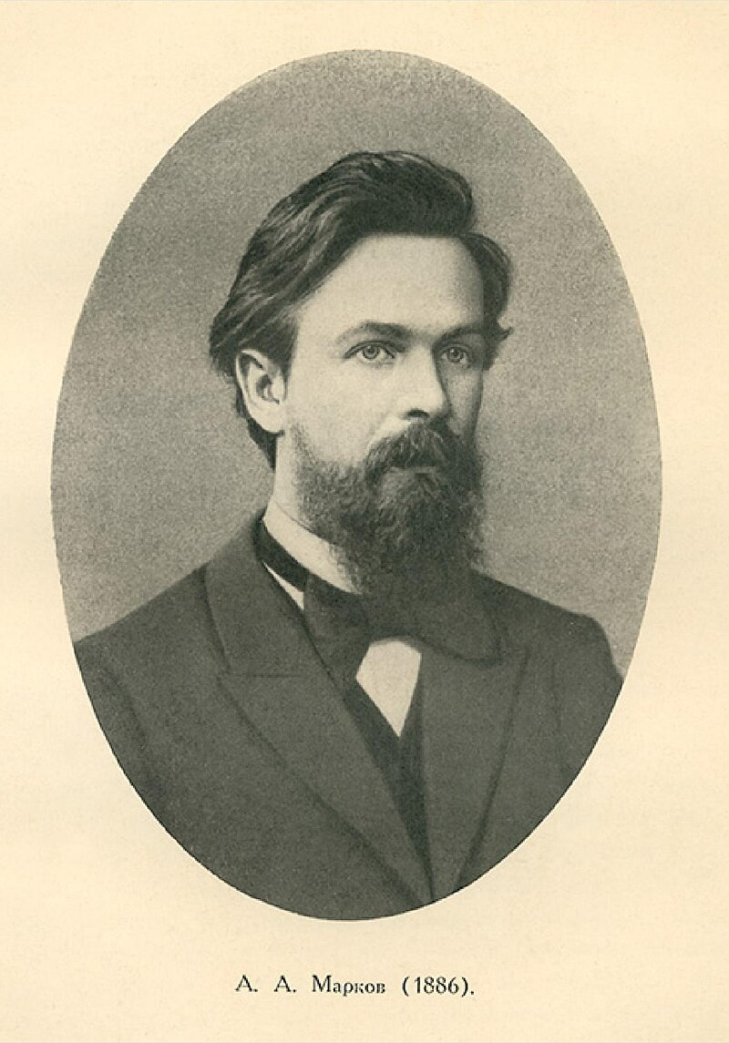
Markov
Markov Chain Monte Carlo
Markov Chain Monte Carlo
Markov Chain Monte Carlo
Markov Chain Monte Carlo
So how do we create the chain?
τ
Start with an initial sample τ.
At each iteration:
1
Sample τ′∼g(⋅∣τ)
e.g. τ′∼N(⋅∣τ,σ2)
2
Accept with probability
pˉ(τ)g(τ′∣τ)pˉ(τ′)g(τ∣τ′)
(otherwise keep τ)
kernel
Markov Chain Monte Carlo
So how do we create the chain?
τ
Start with an initial sample τ.
At each iteration:
1
Sample τ′∼g(⋅∣τ)
e.g. τ′∼N(⋅∣τ,σ2)
2
Accept with probability
pˉ(τ)g(τ′∣τ)pˉ(τ′)g(τ∣τ′)
(otherwise keep τ)
Markov Chain Monte Carlo
So how do we create the chain?
τ
Start with an initial sample τ.
At each iteration:
1
Sample τ′∼g(⋅∣τ)
e.g. τ′∼N(⋅∣τ,σ2)
2
Accept with probability
pˉ(τ)g(τ′∣τ)pˉ(τ′)g(τ∣τ′)
(otherwise keep τ)
Markov Chain Monte Carlo
So how do we create the chain?
τ
Start with an initial sample τ.
At each iteration:
1
Sample τ′∼g(⋅∣τ)
e.g. τ′∼N(⋅∣τ,σ2)
2
Accept with probability
pˉ(τ)g(τ′∣τ)pˉ(τ′)g(τ∣τ′)
(otherwise keep τ)
Markov Chain Monte Carlo
So how do we create the chain?
τ
Start with an initial sample τ.
At each iteration:
1
Sample τ′∼g(⋅∣τ)
e.g. τ′∼N(⋅∣τ,σ2)
2
Accept with probability
pˉ(τ)g(τ′∣τ)pˉ(τ′)g(τ∣τ′)
(otherwise keep τ)
Markov Chain Monte Carlo
So how do we create the chain?
τ
Start with an initial sample τ.
At each iteration:
1
Sample τ′∼g(⋅∣τ)
e.g. τ′∼N(⋅∣τ,σ2)
2
Accept with probability
pˉ(τ)g(τ′∣τ)pˉ(τ′)g(τ∣τ′)
(otherwise keep τ)
Markov Chain Monte Carlo
So how do we create the chain?
τ
Start with an initial sample τ.
At each iteration:
1
Sample τ′∼g(⋅∣τ)
e.g. τ′∼N(⋅∣τ,σ2)
2
Accept with probability
pˉ(τ)g(τ′∣τ)pˉ(τ′)g(τ∣τ′)
(otherwise keep τ)
And so on…
Markov Chain Monte Carlo
So how do we create the chain?
Start with an initial sample τ.
At each iteration:
1
Sample τ′∼g(⋅∣τ)
e.g. τ′∼N(⋅∣τ,σ2)
2
Accept with probability
pˉ(τ)g(τ′∣τ)pˉ(τ′)g(τ∣τ′)
(otherwise keep τ)
And so on…
This process is guaranteed to
converge to the target distribution in
the limit of infinite samples.
converge to the target distribution in
the limit of infinite samples.
Markov Chain Monte Carlo
Some Intuition
Accept with probability
pˉ(τ)g(τ′∣τ)g(τ′∣τ)pˉ(τ′)g(τ∣τ′)g(τ∣τ′)
This process is guaranteed to
converge to the target distribution in
the limit of infinite samples.
converge to the target distribution in
the limit of infinite samples.
The kernel is often chosen to be
symmetric such that
g(τ∣τ′)=g(τ′∣τ).
symmetric such that
g(τ∣τ′)=g(τ′∣τ).
We want to sample from areas of high density more often than areas of low density.
Two cases:
1
pˉ(τ′)≥pˉ(τ)
τ′ is more likely under the target density than τ
pˉ(τ)pˉ(τ′)≥1
Always accept!
2
pˉ(τ′)<pˉ(τ)
τ′ is less likely under the target density than τ
pˉ(τ)pˉ(τ′)<1
Accept with probability proportional to how much less likely it is.
Markov Chain Monte Carlo
Some Intuition
🤔
Still scratching your head?
Markov Chain Monte Carlo
Some Intuition
🤔
Still scratching your head?
Samples1
Initial sample-2.0
Burn in1
Markov Chain Monte Carlo
This all works (converges to the target distribution) in the limit of infinite samples.
Markov Chain Monte Carlo
This all works (converges to the target distribution) in the limit of infinite samples.

We don’t have time for that!
Markov Chain Monte Carlo
This all works (converges to the target distribution) in the limit of infinite samples.
We don’t have time for that!
So we need often use some extra tricks in practice to make it perform better for a finite number of samples.
1
Burn in period
2
Thinning (e.g. only keep every 5th sample)
Deals with the fact that samples at subsequent steps are correlated
3
Smoothing
Markov Chain Monte Carlo
Multiple Failure Modes
Failure if ∣τ∣≥2
Chain starts at τ=−2.1
Chain starts at τ=−2.1
Samples1
Markov Chain Monte Carlo
Smoothing
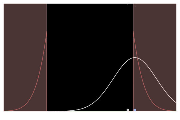

We may need to “help” the algorithm move between failure modes.
We can do this by “smoothing out” the failure distribution.
We can do this by “smoothing out” the failure distribution.
Markov Chain Monte Carlo
Smoothing
We may need to “help” the algorithm move between failure modes.
We can do this by “smoothing out” the failure distribution.
We can do this by “smoothing out” the failure distribution.
Define distance Δ(τ) for each trajectory such that:
Δ(τ)=0
if τ is a failure
Δ(τ)>0
otherwise
e.g. max(ρ(τ,ψ),0)
pˉ(τ∣τ∈/ψ)=1{τ∈/ψ}p(τ)
=1{Δ(τ)=0}p(τ)
1{Δ(τ)=0}≈N(Δ(τ)∣0,ϵ2)
when ϵ is small
0
Δ(τ)
≈
0
Δ(τ)
pˉ(τ∣τ∈/ψ)≈N(Δ(τ)∣0,ϵ2)p(τ)
The smoothed distribution assigns
nonzero probability to successes with
higher probabilities for successes that
are closer to failure.
nonzero probability to successes with
higher probabilities for successes that
are closer to failure.
Markov Chain Monte Carlo
Define distance Δ(τ) for each trajectory such that:
Δ(τ)=0
if τ is a failure
Δ(τ)>0
otherwise
e.g. max(ρ(τ,ψ),0)
pˉ(τ∣τ∈/ψ)=1{τ∈/ψ}p(τ)
=1{Δ(τ)=0}p(τ)
1{Δ(τ)=0}≈N(Δ(τ)∣0,ϵ2)
when ϵ is small
0
Δ(τ)
≈
0
Δ(τ)
pˉ(τ∣τ∈/ψ)≈N(Δ(τ)∣0,ϵ2)p(τ)
The smoothed distribution assigns
nonzero probability to successes with
higher probabilities for successes that
are closer to failure.
nonzero probability to successes with
higher probabilities for successes that
are closer to failure.
The parameter ϵ controls the amount of smoothing applied:
ϵ
∞
nominal trajectory
distribution
distribution
0
no smoothing
Markov Chain Monte Carlo
🤔But won’t we now have a bunch of samples that are not failures?
Yes, but we can just reject them, and we will be left with samples from the failure distribution!
Note: you can think of it as applying
rejection sampling with the smoothed distribution
as the proposal distribution.
rejection sampling with the smoothed distribution
as the proposal distribution.
Markov Chain Monte Carlo
Smoothing
pˉ(τ)=N(Δ(τ)∣0,ϵ2)p(τ)
Δ(τ)=max(2−∣τ∣,0)
Δ(τ)=max(2−∣τ∣,0)
ϵ0.05
Plan for Today
1
Unnormalized Probability Density
2
Rejection Sampling
3
Markov Chain Monte Carlo
4
Tips to Scale Things Up
Tips to Scale Things Up
It is possible to apply these methods to more than just a one-dimensional Gaussian distribution 😀.
Tips to Scale Things Up
It is possible to apply these methods to more than just a one-dimensional Gaussian distribution 😀.
See examples 6.2 and 6.4 to show how we can apply
MCMC and smoothing to the pendulum example.
MCMC and smoothing to the pendulum example.
Other methods that help:
1
Some MCMC methods use gradients of the likelihood to define the kernel, which can
lead to better performance (e.g. MALA in section 6.3.3, HMC, NUTS)
lead to better performance (e.g. MALA in section 6.3.3, HMC, NUTS)
2
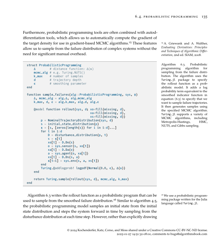
Probabilistic programming allows us to specify probabilistic models as computer
programs in a way that allows inference to be performed automatically.
programs in a way that allows inference to be performed automatically.
Advanced
topics
topics
Tips to Scale Things Up
Inverted pendulum: MCMC with a smoothed failure distribution (kmax=50,000, keep every 500th)
Smoothing ϵ0.15
Tips to Scale Things Up
2
Probabilistic programming allows us to specify probabilistic models as computer
programs in a way that allows inference to be performed automatically.
programs in a way that allows inference to be performed automatically.
😲
Plan for Today
1
Unnormalized Probability Density
2
Rejection Sampling
3
Markov Chain Monte Carlo
4
Tips to Scale Things Up