
AA228V/CS238V
Validation of Safety-Critical Systems
Validation of Safety-Critical Systems
Lecture 05/06: Falsification Through Optimization
Sydney Katz (smkatz@stanford.edu)
Sydney Katz (smkatz@stanford.edu)
Falsification = Systematically Finding Failures
Falsification = Systematically Finding Failures
Why find failures?
To inform future design decisions.

Enhance system sensors

Change agent’s policy

Revise system requirements

Adapt training of human operators

Recognize as limitations

Abandon the project
On a happy note…



A Baseline Approach
Direct Sampling
Direct Sampling
Perception noise σ0.10
Depth d41
Number of rollouts m50
Direct Samplingmay perform poorly for systems with rare failure events.
Direct Samplingmay perform poorly for systems with rare failure events.
Direct Samplingmay perform poorly for systems with rare failure events.
Geometric distribution:
P(k)=(1−pfail)k−1pfail
P(k)=(1−pfail)k−1pfail
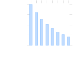
Pfail=0.2
Direct Samplingmay perform poorly for systems with rare failure events.
Geometric distribution:
P(k)=(1−pfail)k−1pfail
P(k)=(1−pfail)k−1pfail
Pfail=0.2
The expected value of this distribution is
E[k]=1/Pfail
In other words, it should require 1/Pfail
simulations on average to find a single
failure event.
simulations on average to find a single
failure event.
Direct Samplingmay perform poorly for systems with rare failure events.
In other words, it should require 1/Pfail
simulations on average to find a single
failure event.
simulations on average to find a single
failure event.
For systems with rare failure events, Pfail is really low.

e.g. imagine an aircraft collision avoidance system with Pfail≈10−9
We would need an average of 1 billion simulations to observe a single failure!
🤔
We are going to need a better way.
Plan for Today
1
Direct Sampling
2
Disturbances
3
Fuzzing
4
Optimization
This is what I would start with for Project 1!
Plan for Today
1
Direct Sampling
2
Disturbances
3
Fuzzing
4
Optimization
This (and/or what we learn Thursday) is what I would do to
improve my leaderboard score.
improve my leaderboard score.
🤔
Direct Samplingmay perform poorly for systems with rare failure events.
We can instead systematically search for failures by taking control of the sources of randomness in a system using
Disturbances
To incorporate disturbances into a system, we need to rewrite its agent, environment, and sensor models:
a∼π(⋅∣o), s′∼T(⋅∣s,a), and o∼O(⋅∣s).
a∼π(⋅∣o), s′∼T(⋅∣s,a), and o∼O(⋅∣s).
To incorporate disturbances into a system, we need to rewrite its agent, environment, and sensor models:
a∼π(⋅∣o), s′∼T(⋅∣s,a), and o∼O(⋅∣s).
a∼π(⋅∣o), s′∼T(⋅∣s,a), and o∼O(⋅∣s).
To incorporate disturbances into a system, we need to rewrite its agent, environment, and sensor models:
a∼π(⋅∣o), s′∼T(⋅∣s,a), and o∼O(⋅∣s).
a∼π(⋅∣o), s′∼T(⋅∣s,a), and o∼O(⋅∣s).
o∼O(⋅∣s)
To incorporate disturbances into a system, we need to rewrite its agent, environment, and sensor models:
a∼π(⋅∣o), s′∼T(⋅∣s,a), and o∼O(⋅∣s).
a∼π(⋅∣o), s′∼T(⋅∣s,a), and o∼O(⋅∣s).
o∼O(⋅∣s)
rewrite
o=O(s,xo),xo∼Do(⋅∣s)
deterministic
function
function
disturbance
distribution
distribution
disturbance
o∼O(⋅∣s)
rewrite
o=O(s,xo),xo∼Do(⋅∣s)
Example
Recall the inverted pendulum observation model: o∼N(⋅∣s,Σ)
We can rewrite with disturbances as follows:
o=s+xo, xo∼N(⋅∣0,Σ)
In this case, the disturbance represents the “observation noise” added to the true state.
The observation noise is sampled from a disturbance distribution centered at zero (no
noise) with covariance Σ.
noise) with covariance Σ.

xo
Note: the model with disturbances still represents the same process. We have just
separated out the stochastic components so that we can control them!
separated out the stochastic components so that we can control them!
Sensor
o∼O(⋅∣s)
rewrite
o=O(s,xo),xo∼Do(⋅∣s)
Agent
a∼π(⋅∣o)
rewrite
a=π(o,xa),xa∼Da(⋅∣o)
Environment
s′∼T(⋅∣s,a)
rewrite
s′=T(s,a,xs),xs∼Ds(⋅∣s,a)
Sensor
o∼O(⋅∣s)
rewrite
o=O(s,xo),xo∼Do(⋅∣s)
Agent
a∼π(⋅∣o)
rewrite
a=π(o,xa),xa∼Da(⋅∣o)
Environment
s′∼T(⋅∣s,a)
rewrite
s′=T(s,a,xs),xs∼Ds(⋅∣s,a)
Disturbance x
xaxsxo
Disturbance distribution D
Do(⋅∣s)Da(⋅∣o)Ds(⋅∣s,a)
“disturbution”
Sensor
o∼O(⋅∣s)
rewrite
o=O(s,xo),xo∼Do(⋅∣s)
Agent
a∼π(⋅∣o)
rewrite
a=π(o,xa),xa∼Da(⋅∣o)
Environment
s′∼T(⋅∣s,a)
rewrite
s′=T(s,a,xs),xs∼Ds(⋅∣s,a)

o∼N(⋅∣s,Σ)
o=s+xo, xo∼N(⋅∣0,Σ)
π(a∣o)={10if a=−15.0θ−8.0ωotherwise
a=−15.0θ^−8.0ω^
*Note: no xa because the
agent is deterministic!
agent is deterministic!
T(s′∣s,a)=⎩⎨⎧10if s′=[θ+ωΔtω+(2l3gsinθ+ml23a)Δt]otherwise
s′=[θ+ωΔtω+(2l3gsinθ+ml23a)Δt]
*Note: no xs because the
environment is deterministic!
environment is deterministic!
Disturbance x
xaxsxo
Disturbance distribution D
Do(⋅∣s)Da(⋅∣o)Ds(⋅∣s,a)
Disturbance x
xaxsxo
Disturbance distribution D
Do(⋅∣s)Da(⋅∣o)Ds(⋅∣s,a)
Disturbance x
xaxsxo
Disturbance distribution D
Do(⋅∣s)Da(⋅∣o)Ds(⋅∣s,a)
Disturbance x
xaxsxo
Disturbance distribution D
Do(⋅∣s)Da(⋅∣o)Ds(⋅∣s,a)
θ
ω
s=[0.3,0.1]
Disturbance x
xaxsxo
Disturbance distribution D
Do(⋅∣s)Da(⋅∣o)Ds(⋅∣s,a)
θ
ω
s=[0.3,0.1]
o=s+xo,xo∼N(⋅∣0,Σ)

xθ
xω

xo=[0.2,0.25]
Disturbance x
xaxsxo
Disturbance distribution D
Do(⋅∣s)Da(⋅∣o)Ds(⋅∣s,a)
θ
ω
s=[0.3,0.1]
xo=[0.2,0.25]
o=s+xo,xo∼N(⋅∣0,Σ)
Disturbance x
xaxsxo
Disturbance distribution D
Do(⋅∣s)Da(⋅∣o)Ds(⋅∣s,a)
s=[0.3,0.1]
xo=[0.2,0.25]
o=s+xo,xo∼N(⋅∣0,Σ)
θ+xθ
ω+xω
o=[0.5,0.35]
Disturbance x
xaxsxo
Disturbance distribution D
Do(⋅∣s)Da(⋅∣o)Ds(⋅∣s,a)
s=[0.3,0.1]
xo=[0.2,0.25]
o=[0.5,0.35]
deterministic for the pendulum!
Disturbance x
xaxsxo
Disturbance distribution D
Do(⋅∣s)Da(⋅∣o)Ds(⋅∣s,a)
s=[0.3,0.1]
xo=[0.2,0.25]
o=[0.5,0.35]
deterministic for the pendulum!
a=−15.0θ^−8.0ω^
a=−15.0(0.5)−8.0(0.35)=−9.9
Disturbance x
xaxsxo
Disturbance distribution D
Do(⋅∣s)Da(⋅∣o)Ds(⋅∣s,a)
s=[0.3,0.1]
xo=[0.2,0.25]
o=[0.5,0.35]
deterministic for the pendulum!
a=−15.0(0.5)−8.0(0.35)=−9.9
deterministic for the pendulum!
Disturbance x
xaxsxo
Disturbance distribution D
Do(⋅∣s)Da(⋅∣o)Ds(⋅∣s,a)
s=[0.3,0.1]
xo=[0.2,0.25]
o=[0.5,0.35]
deterministic for the pendulum!
a=−15.0(0.5)−8.0(0.35)=−9.9
deterministic for the pendulum!
s′=[θ+ωΔtω+(2l3gsinθ+ml23a)Δt]
s′=[0.31,−1.38]
Disturbance x
xaxsxo
Disturbance distribution D
Do(⋅∣s)Da(⋅∣o)Ds(⋅∣s,a)
s=[0.3,0.1]
xo=[0.2,0.25]
o=[0.5,0.35]
deterministic for the pendulum!
a=−15.0(0.5)−8.0(0.35)=−9.9
deterministic for the pendulum!
s′=[0.31,−1.38]
record everything
that happened
that happened
Disturbance x
xaxsxo
Disturbance distribution D
Do(⋅∣s)Da(⋅∣o)Ds(⋅∣s,a)
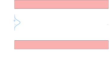
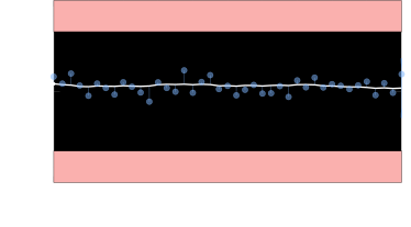
We can use the idea of disturbances to explicitly define the distribution over trajectories for a system.
We can use the idea of disturbances to explicitly define the distribution over trajectories for a system.
There are two sources of randomness in a trajectory rollout:
1
the initial state
2
the disturbance applied at each time step


We can use the idea of disturbances to explicitly define the distribution over trajectories for a system.
There are two sources of randomness in a trajectory rollout:
1
the initial state
2
the disturbance applied at each time step

We can use the idea of disturbances to explicitly define the distribution over trajectories for a system.
There are two sources of randomness in a trajectory rollout:
1
the initial state
2
the disturbance applied at each time step
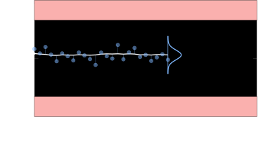
Trajectory Distribution
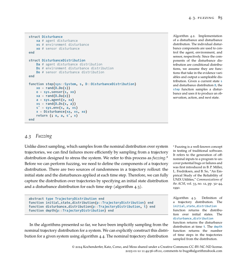
We can use the idea of disturbances to explicitly define the distribution over trajectories for a system.
There are two sources of randomness in a trajectory rollout:
1
the initial state
2
the disturbance applied at each time step
Trajectory Distribution
We can use the idea of disturbances to explicitly define the distribution over trajectories for a system.
There are two sources of randomness in a trajectory rollout:
1
the initial state
2
the disturbance applied at each time step
Trajectory Distribution
We can use the idea of disturbances to explicitly define the distribution over trajectories for a system.
There are two sources of randomness in a trajectory rollout:
1
the initial state
2
the disturbance applied at each time step
Trajectory Distribution
We can use the idea of disturbances to explicitly define the distribution over trajectories for a system.
There are two sources of randomness in a trajectory rollout:
1
the initial state
2
the disturbance applied at each time step
Trajectory Distribution
Sampling a Trajectory Distribution: Rollout
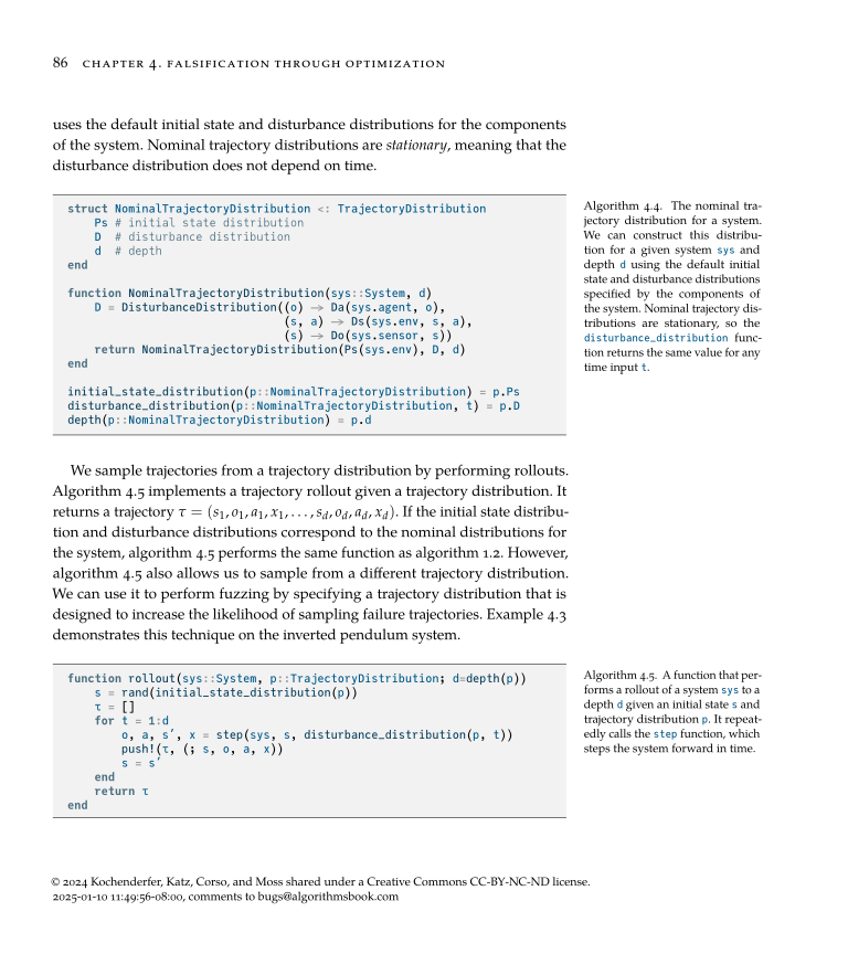
We can use the idea of disturbances to explicitly define the distribution over trajectories for a system.
There are two sources of randomness in a trajectory rollout:
Trajectory Distribution
Sampling a Trajectory Distribution: Rollout
🤔
Wait.. didn’t we already see a different algorithm for rollout in the intro lecture?
Sampling a Trajectory Distribution: Rollout
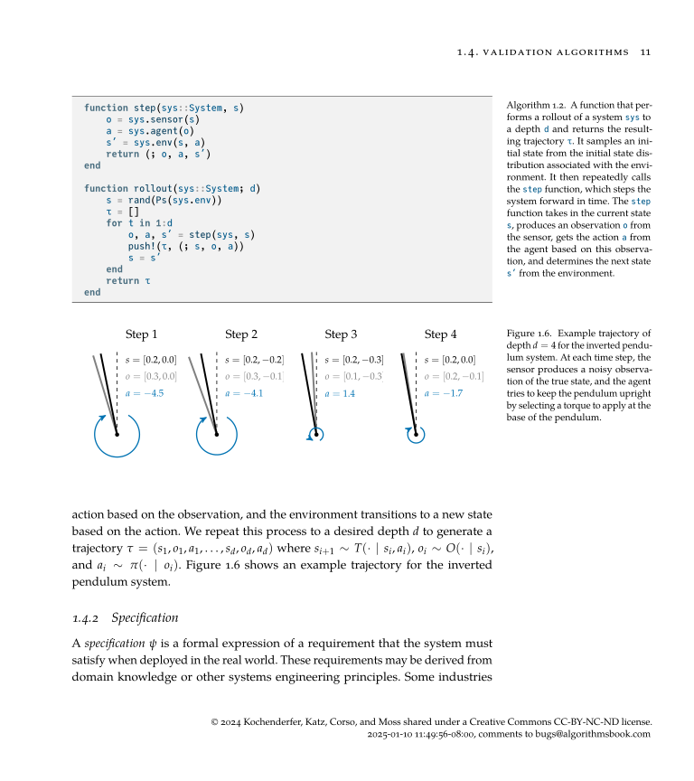
Rollout from Introduction Lecture
This version of rollout is
implicitly sampling from the
nominal trajectory distribution
for the system.
implicitly sampling from the
nominal trajectory distribution
for the system.
Thenominal trajectory distributionrepresents the distribution over trajectories that we expect to observe in the real world.
Thenominal trajectory distributionrepresents the distribution over trajectories that we expect to observe in the real world.
Note:
- Every agent has a nominal Da implemented
- Every environment has a nominal Ps and Ds implemented
- Every sensor has a nominal Do implemented
The nominal models come from data/expert knowledge from
the real world (see chapter 2!).
the real world (see chapter 2!).
Pendulum example: the nominal trajectory distribution
PsU([−16π,16π])×U([−1,1])Da(⋅∣o)DeterministicDs(⋅∣s,a)DeterministicDo(⋅∣s)N(0,0.12I)
🤔
Wait.. didn’t we already see a different algorithm for rollout in the intro lecture?
Sampling a Trajectory Distribution: Rollout
Rollout from Introduction Lecture
This version of rollout is
implicitly sampling from the
nominal trajectory distribution
for the system.
implicitly sampling from the
nominal trajectory distribution
for the system.
=
Plan for Today
1
Direct Sampling
2
Disturbances
3
Fuzzing
4
Optimization
This is what I would start with for Project 1!
Fuzzing
Input a different (not nominal) trajectory distribution into this
function — one that is more likely to cause failures.
function — one that is more likely to cause failures.
e.g. for the inverted pendulum, we could use a disturbance distribution with
higher perception noise than the nominal distribution
higher perception noise than the nominal distribution
Fuzzing
Nominal perception noise
σ=0.1
σ=0.1
Fuzzing noise σfuzz0.10
Rollouts m50
Another happy note…


Plan for Today
1
Direct Sampling
2
Disturbances
3
Fuzzing
4
Optimization
This (and/or what we learn next week) is what I would do to
improve my leaderboard score.
improve my leaderboard score.
Optimization
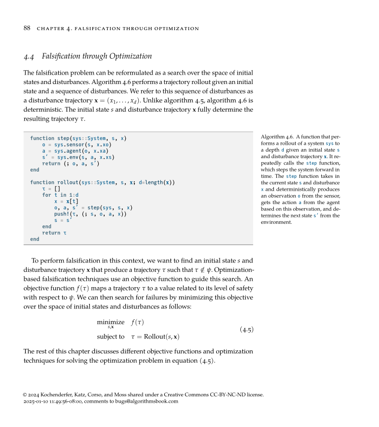
Our goal is to systematically search over initial states and sequences of disturbances to find failure trajectories.
Optimization
Our goal is to systematically search over initial states and sequences of disturbances to find failure trajectories.
Optimization
Our goal is to systematically search over initial states and sequences of disturbances to find failure trajectories.
s
Optimization
Our goal is to systematically search over initial states and sequences of disturbances to find failure trajectories.
s
, x
minimize
f(τ)
subject to
τ=Rollout(s,x)
objective function that represents
“closeness to failure”
“closeness to failure”
Optimization
Our goal is to systematically search over initial states and sequences of disturbances to find failure trajectories.
s
, x
minimize
f(τ)
subject to
τ=Rollout(s,x)
objective function that represents
“closeness to failure”
“closeness to failure”
Optimization
Our goal is to systematically search over initial states and sequences of disturbances to find failure trajectories.
f(τ)
f(τ)
objective function that represents
“closeness to failure”
“closeness to failure”
🤔
What metric from chapter 3 reminds you of “closeness to failure”?
Robustness!
(or if our optimization algorithm needs gradients, smooth robustness)
Optimization
Our goal is to systematically search over initial states and sequences of disturbances to find failure trajectories.
f(τ)
objective function that represents
“closeness to failure”
“closeness to failure”
🤔
What metric from chapter 3 reminds you of “closeness to failure”?
Robustness!
(or if our optimization algorithm needs gradients, smooth robustness)
f(τ)=ρ(τ,ψ)
🤔
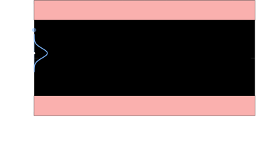
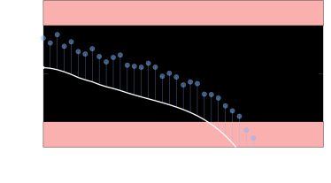
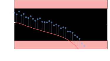
What might be a problem with the robustness objective?
We might get very unlikely trajectories…
Optimization
Our goal is to systematically search over initial states and sequences of disturbances to find failure trajectories.
🤔
What might be a problem with the robustness objective?
We might get very unlikely trajectories…

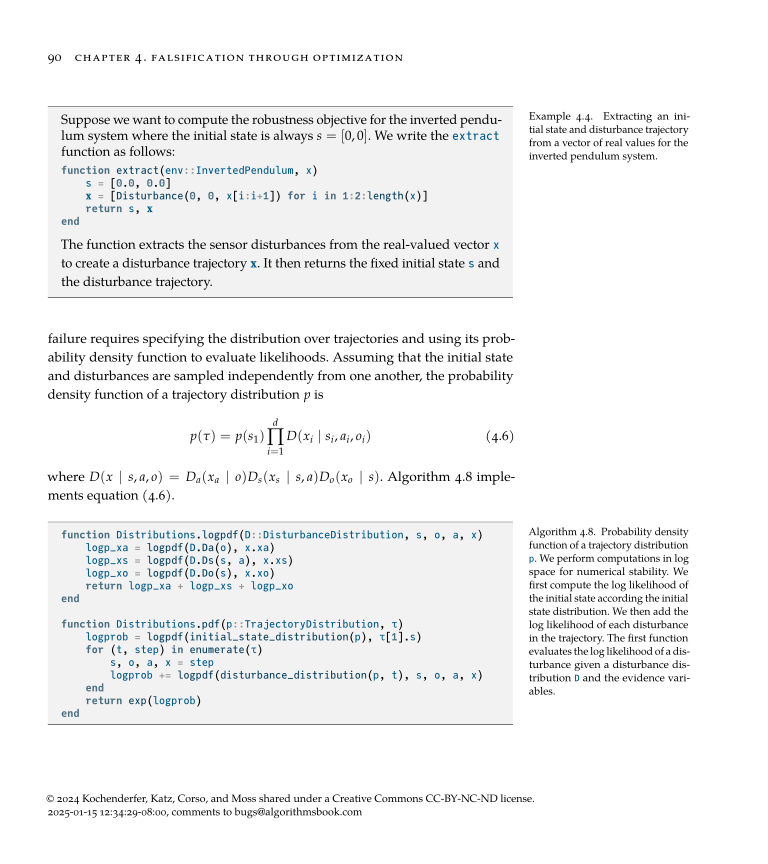
incorporate likelihood
into the objective
into the objective
incorporate likelihood
into the objective
into the objective
How do we evaluate the likelihood of a trajectory?
The likelihood of the trajectory is the likelihood of the initial state and all disturbances in the trajectory occurring.
p(τ)=
p(s1)
incorporate likelihood
into the objective
into the objective
How do we evaluate the likelihood of a trajectory?
The likelihood of the trajectory is the likelihood of the initial state and all disturbances in the trajectory occurring.
p(τ)=p(s1)
incorporate likelihood
into the objective
into the objective
How do we evaluate the likelihood of a trajectory?
The likelihood of the trajectory is the likelihood of the initial state and all disturbances in the trajectory occurring.
p(τ)=p(s1)
D(x1∣s1,a1,o1)
incorporate likelihood
into the objective
into the objective
How do we evaluate the likelihood of a trajectory?
The likelihood of the trajectory is the likelihood of the initial state and all disturbances in the trajectory occurring.
p(τ)=p(s1)D(x1∣s1,a1,o1)
incorporate likelihood
into the objective
into the objective
How do we evaluate the likelihood of a trajectory?
The likelihood of the trajectory is the likelihood of the initial state and all disturbances in the trajectory occurring.
p(τ)=p(s1)D(x1∣s1,a1,o1)
D(x2∣s2,a2,o2)
incorporate likelihood
into the objective
into the objective
How do we evaluate the likelihood of a trajectory?
The likelihood of the trajectory is the likelihood of the initial state and all disturbances in the trajectory occurring.
p(τ)=p(s1)D(x1∣s1,a1,o1)D(x2∣s2,a2,o2)
incorporate likelihood
into the objective
into the objective
How do we evaluate the likelihood of a trajectory?
The likelihood of the trajectory is the likelihood of the initial state and all disturbances in the trajectory occurring.
p(τ)=p(s1)D(x1∣s1,a1,o1)D(x2∣s2,a2,o2)⋯D(xd∣sd,ad,od)
incorporate likelihood
into the objective
into the objective
How do we evaluate the likelihood of a trajectory?
The likelihood of the trajectory is the likelihood of the initial state and all disturbances in the trajectory occurring.
p(τ)=p(s1)D(x1∣s1,a1,o1)D(x2∣s2,a2,o2)⋯D(xd∣sd,ad,od)
D(x∣s,a,o)=Da(xa∣o)Ds(xs∣s,a)Do(xo∣s)
log
log
incorporate likelihood
into the objective
into the objective
New Objective:
f(τ)={−p(τ)ρ(τ,ψ)if τ∈/ψotherwise
1
The trajectory τ is a failure.
“Make the failure trajectory more likely”
2
The trajectory τ is not a failure.
“Move the trajectory closer to a failure”
incorporate likelihood
into the objective
into the objective
Previous Objective:
f(τ)=ρ(τ,ψ)
New Objective:
f(τ)={−p(τ)ρ(τ,ψ)if τ∈/ψotherwise
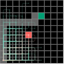
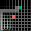
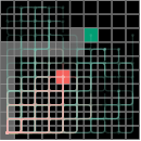
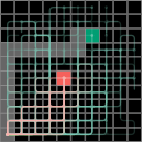
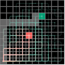
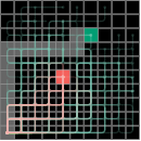
incorporate likelihood
into the objective
into the objective
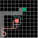
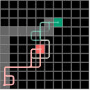
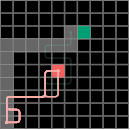
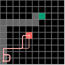
Previous Objective:
f(τ)=ρ(τ,ψ)
New Objective:
f(τ)={−p(τ)ρ(τ,ψ)if τ∈/ψotherwise
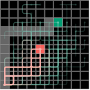
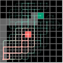
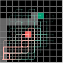
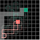
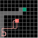
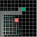
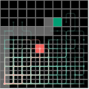
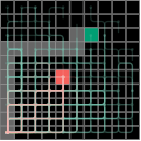
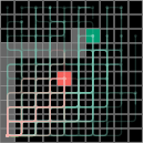
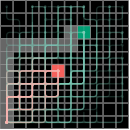
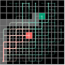
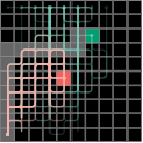
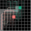
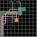
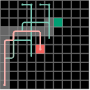
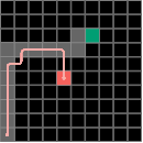
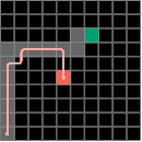
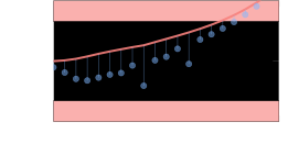
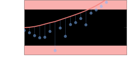
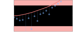
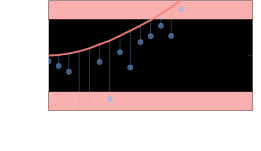
Iteration 1
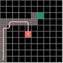
Iteration 5
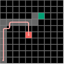
Iteration 8
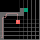
Converged
incorporate likelihood
into the objective
into the objective
f(τ)={−p(τ)ρ(τ,ψ)if τ∈/ψotherwise
Some Notes on This Objective
We must ensure that failures never have a
higher objective value than successes.
higher objective value than successes.

No problem! ρ(τ,ψ)≥0 for successes
and −p(τ) is always less than 0.
and −p(τ) is always less than 0.
…but p(τ) is often really small causing
numerical stability issues
numerical stability issues
…so we want to use log-likelihood instead, but
this breaks the first requirement because log
likelihood can be less than 0!
this breaks the first requirement because log
likelihood can be less than 0!
…so sometimes a different objective works
better in practice (see next slide)
better in practice (see next slide)
incorporate likelihood
into the objective
into the objective
f(τ)={−p(τ)ρ(τ,ψ)if τ∈/ψotherwise
f(τ)=ρ(τ,ψ)−λlog(p(τ))
robustness
*tends to be more numerically stable
incorporate likelihood
into the objective
into the objective
f(τ)={−p(τ)ρ(τ,ψ)if τ∈/ψotherwise
f(τ)=ρ(τ,ψ)−λlog(p(τ))
log likelihood
*tends to be more numerically stable
incorporate likelihood
into the objective
into the objective
f(τ)={−p(τ)ρ(τ,ψ)if τ∈/ψotherwise
f(τ)=ρ(τ,ψ)−λlog(p(τ))
weighting
parameter
parameter
*tends to be more numerically stable
Then we optimize!
Then we optimize!
Then we optimize!
Objective Function
Optimizer
Then we optimize!
Objective Function
Optimizer
1
f(τ)=ρ(τ,ψ)
2
f(τ)={−p(τ)ρ(τ,ψ)if τ∈/ψotherwise
3
f(τ)=ρ(τ,ψ)−λlog(p(τ))
Then we optimize!
Objective Function
Optimizer
1
f(τ)=ρ(τ,ψ)
2
f(τ)={−p(τ)ρ(τ,ψ)if τ∈/ψotherwise
3
f(τ)=ρ(τ,ψ)−λlog(p(τ))
Optimization
Algorithm
Algorithm
Objective
Parameters
Optimum
Optimization
Algorithm
Algorithm
Objective
Parameters
Optimum
s,x
Local Descent Methods
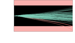
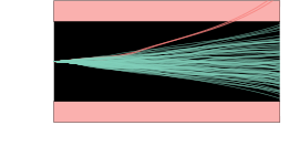
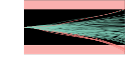
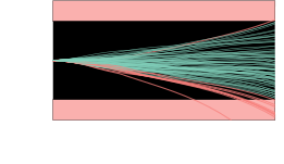
Population Methods
x
f(x)
Optimization
Algorithm
Algorithm
Objective
Parameters
Optimum
s,x
Local Descent Methods
Population Methods
x
f(x)
x
f(x)
Optimization
Algorithm
Algorithm
Objective
Parameters
Optimum
s,x
Local Descent Methods
Population Methods
x
f(x)
x
f(x)
first-order and
second-order
second-order
e.g. gradient descent,
ADAM, LBFGS
ADAM, LBFGS
 !
gradients
required!
required!
zero-order
(direct methods)
(direct methods)
e.g. Hooke-Jeeves,
Nelder-Mead
Nelder-Mead
work for black-
box systems!
box systems!
Optimization
Algorithm
Algorithm
Objective
Parameters
Optimum
s,x
Local Descent Methods
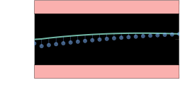
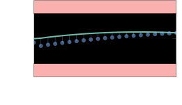
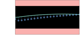
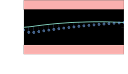
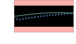
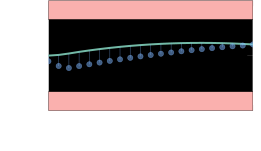
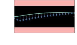
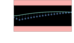
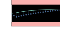
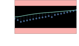
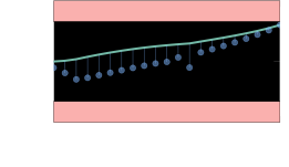
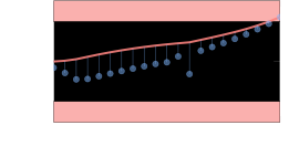
Optimization
Algorithm
Algorithm
Objective
Parameters
Optimum
s,x
Local Descent Methods
Population Methods
x
f(x)
x
f(x)
first-order and
second-order
second-order
e.g. gradient descent,
ADAM, LBFGS
ADAM, LBFGS
!gradients
required!
required!
zero-order
(direct methods)
(direct methods)
e.g. Hooke-Jeeves,
Nelder-Mead
Nelder-Mead
work for black-
box systems!
box systems!
Optimization
Algorithm
Algorithm
Objective
Parameters
Optimum
s,x
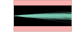
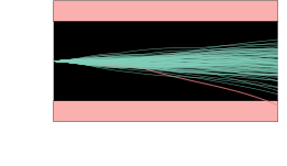
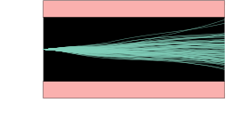
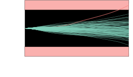
Population Methods
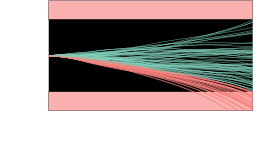
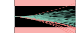
Optimization
Algorithm
Algorithm
Objective
Parameters
Optimum
s,x
Local Descent Methods
Population Methods
x
f(x)
x
f(x)
first-order and
second-order
second-order
e.g. gradient descent,
ADAM, LBFGS
ADAM, LBFGS
!gradients
required!
required!
zero-order
(direct methods)
(direct methods)
e.g. Hooke-Jeeves,
Nelder-Mead
Nelder-Mead
work for black-
box systems!
box systems!
Then we optimize!
Objective Function
Optimizer
1
f(τ)=ρ(τ,ψ)
2
f(τ)={−p(τ)ρ(τ,ψ)if τ∈/ψotherwise
3
f(τ)=ρ(τ,ψ)−λlog(p(τ))
Optimization
Algorithm
Algorithm
Objective
Parameters
Optimum
Take AA222/CS361 for more details!!!
Plan for Today
1
Direct Sampling
2
Disturbances
3
Fuzzing
4
Optimization
This is what I would start with for Project 1!
This (and/or what we learn Thursday) is what I would do to
improve my leaderboard score.
improve my leaderboard score.