
AA228V/CS238V
Validation of Safety-Critical Systems
Validation of Safety-Critical Systems
Lecture 02/03: System Modeling
Sydney Katz (smkatz@stanford.edu)
Sydney Katz (smkatz@stanford.edu)
***
AA222/CS361
AA228/CS238
AA228V/CS238V
*In a controlled, safe environment such as a simulation instead of the real world
*In a controlled, safe environment such as a simulation instead of the real world
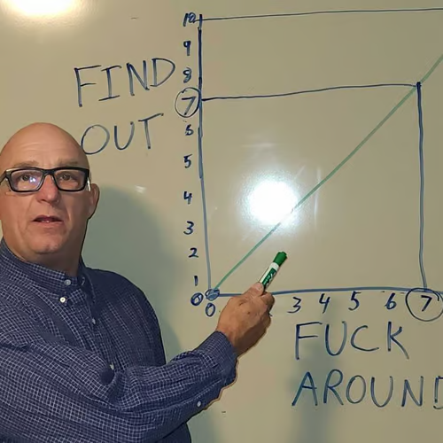
… unlike these people.


We don’t want to find out in the real world!
We do want to find out in simulation!
Today, we will discuss ways to model systems so that
we can simulate them for offline validation.
we can simulate them for offline validation.
Plan for Today
1
General Thoughts on Models
2
Steps for Building Models
A
Select a Model Class
B
Select the Parameters for the Model Class
C
Validate the Model
General Thoughts on Models
There are many different types of models/simulators.
They don’t even have to be on the computer!

We will focus on computational models in this class.
General Thoughts on Models
Models vary in complexity.
flight
h′ = h + ḣΔt
ḣ′ = ḣ + ḧΔt
ḣ′ = ḣ + ḧΔt
General Thoughts on Models
Models vary in complexity.
flight

General Thoughts on Models
Models vary in complexity.
flight
h′ = h + ḣΔt
ḣ′ = ḣ + ḧΔt
ḣ′ = ḣ + ḧΔt
low
complexity
complexity
high
complexity
complexity
We want to pick the model that is just complex enough to capture what matters.
General Thoughts on Models
Models vary in complexity.
flight
h′ = h + ḣΔt
ḣ′ = ḣ + ḧΔt
ḣ′ = ḣ + ḧΔt
low
complexity
complexity
high
complexity
complexity
We want to pick the model that is just complex enough to capture what matters.
“Everything should be as simple as possible, but not simpler.”
— Albert Einstein
(maybe)
(maybe)
General Thoughts on Models
Models can be…
White Box
flight
h′ = h + ḣΔt
ḣ′ = ḣ + ḧΔt
ḣ′ = ḣ + ḧΔt
Black Box
flight
or
General Thoughts on Models
Models can be…
White Box
Gray Box
Black Box
flight
flight
flight
h′ = h + ḣΔt
ḣ′ = ḣ + ḧΔt
ḣ′ = ḣ + ḧΔt
or
or
General Thoughts on Models
Key Challenges
1Model needs to be expressive enough to capture all possible scenarios the system may encounter.
How can I capture all possible scenarios my <insert crazy complex system here> will end up in?
… I don’t even know what they all are!
Yeah, it’s a problem. 😬
But there is some hope! Stay tuned for the runtime monitoring chapter.
General Thoughts on Models
Key Challenges
1Model needs to be expressive enough to capture all possible scenarios the system may encounter.
2Requires data and/or expert knowledge.
3Need to select an objective and optimization technique to find model parameters.
“All models are wrong, but some are useful.”
— British statistician George Box (for real)
Plan for Today
1
General Thoughts on Models
2
Steps for Building Models
A
Select a Model Class
B
Select the Parameters for the Model Class
C
Validate the Model
Select a Model Class
We are going to focus on creating probabilistic models.
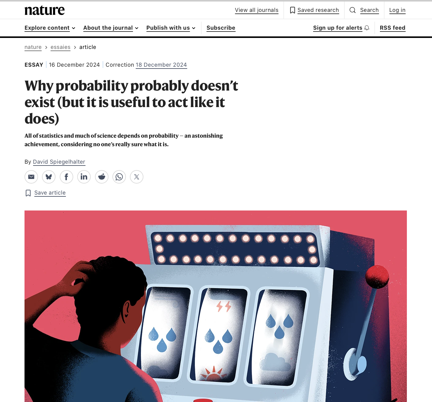
“All of statistics and much of science depends on probability — an astonishing achievement, considering no one’s really sure what it is.”
— David Spiegelhalter, Nature (2024)
Select a Model Class
We are going to focus on creating probabilistic models.
The probability of a particular outcome is a number between zero and one that quantifies the likelihood of that outcome occurring, relative to all possible outcomes.
Select a Model Class
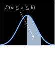
A common type of model class is a probability distribution, which is a function that assigns probabilities to different outcomes.
Discrete Distributions
Continuous Distributions
Probability Mass Function P(x)
Probability Density Function p(x)
∑xP(x)=1
∫−∞∞p(x)dx=1
0≤P(x)≤1
p(x)≥0
SELECT A MODEL CLASS
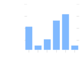
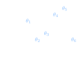
We often represent probability distributions using a set of parameters θ.
SELECT A MODEL CLASS
We often represent probability distributions using a set of parameters θ.
θ=[μ,σ]
SELECT A MODEL CLASS
Main consideration when selecting a model class:
It needs to be “expressive enough.”
i.e. there is some setting of the model parameters for which the model will fit the data well
SELECT A MODEL CLASS
Gaussian Distribution
μ{{ muTxt }}
σ{{ sigTxt }}
We can fit data set 1 well with a Gaussian, but not data set 2, because data set 2 is multimodal.
SELECT A MODEL CLASS
We can fit data set 1 well with a Gaussian, but not data set 2, because data set 2 is multimodal.
Idea: combine several simple distributions into one more expressive distribution.
A Gaussian mixture model is a weighted sum of Gaussians:
p(x)=∑iwiN(x∣μi,σi2),∑iwi=1
SELECT A MODEL CLASS
Gaussian Mixture
p(x)=w1N(x∣μ1,σ12)+w2N(x∣μ2,σ22)
μ1{{ mu1Txt }}
σ1{{ sig1Txt }}
μ2{{ mu2Txt }}
σ2{{ sig2Txt }}
w2=1−w1{{ wTxt }}
SELECT A MODEL CLASS
Single Gaussianpoor fit
If a simple distribution does not fit the data well for any setting of its parameters, we need a more complex model class.
Gaussian Mixturegood fit
One way to create more complex distributions is to use a weighted mixture of simpler distributions.
Another way to create a more complex model class is by applying a functional transformation to a simple distribution.
SELECT A MODEL CLASS
Another way to create a more complex model class is by applying a functional transformation to a simple distribution.
Start with a distribution we know:
Z∼N(0,12)
10,000 samples of Z, with its density
SELECT A MODEL CLASS
Apply a function f to every sample to get a new variable X:
samples of Z
x=f(z)=3z
transformed samples of X
SELECT A MODEL CLASS
We just turned a unimodal distribution into a multimodal one!
SELECT A MODEL CLASS
What is the probability density of this new distribution?
Z∼pz(⋅),X∼px(⋅),x=f(z)
If f is invertible and differentiable, then
px(x)=pz(g(x))∣g′(x)∣
where g is the inverse of f.
g(x)=x3,g′(x)=3x2
px(x)=N(x3∣0,12)⋅3x2
SELECT A MODEL CLASS
Does it match the samples?
px(x)=N(x3∣0,12)⋅3x2
Note: This formula requires f to be differentiable and invertible!
px(x)=pz(g(x))∣g′(x)∣
SELECT A MODEL CLASS
We can still apply a functional transformation that is not differentiable and invertible! We just won’t be able to calculate the resulting PDF.
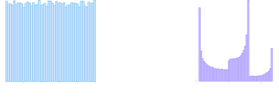
samples from a pseudorandom number generator
transformed samples
We call models represented in this way generative models.
SELECT A MODEL CLASS
We call models represented in this way generative models.
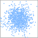
f(x)=neural network
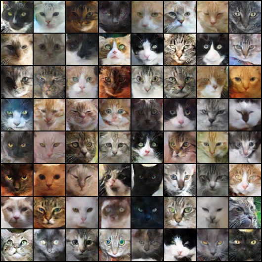
Credit: ajolicoeur.ca/cats

To throw in some buzz words: generative adversarial networks (GANs), variational autoencoders (VAEs), diffusion models, etc.
SELECT A MODEL CLASS
If we have multiple variables involved, we are interested in joint or conditional distributions.
SELECT A MODEL CLASS
joint distribution: probability distribution over multiple variables.
(multivariate distribution)
represents the likelihood of multiple outcomes occurring simultaneously
Discrete: P(x,y)
e.g. table representation
x
y
P(x,y)
0
0
0.1
0
1
0.2
1
0
0.5
1
1
0.2
Continuous: p(x,y)
e.g. multivariate Gaussian

μ
Σ=[1001]

μ
Σ=[10.50.51]

μ
Σ=[1−0.8−0.81]
SELECT A MODEL CLASS
Multivariate Gaussian
Σx{{ SxTxt }}
Σy{{ SyTxt }}
Σxy{{ SxyTxt }}
Σ=
{{ SxTxt }}{{ SxyTxt }}{{ SxyTxt }}{{ SyTxt }}
Not a valid covariance: need Σxy² < ΣxΣy
SELECT A MODEL CLASS
joint distribution: probability distribution over multiple variables.
(multivariate distribution)
represents the likelihood of multiple outcomes occurring simultaneously
Note: If two variables are independent, then P(x,y)=P(x)P(y). Otherwise, this is not the case.
SELECT A MODEL CLASS
Note: If two variables are independent, then P(x,y)=P(x)P(y). Otherwise, this is not the case.
Fun aside: what is the probability that four textbook authors have 0, 0, 4, and 5 wisdom teeth?

SELECT A MODEL CLASS
Fun aside: what is the probability that four textbook authors have 0, 0, 4, and 5 wisdom teeth?
From a few minutes of googling, guessing, and asking ChatGPT. Take these with a grain of salt.
1Find every combination of four counts that adds up to the total.
2Sum the product of their probabilities.
Total = {{ tnTxt }}
SELECT A MODEL CLASS
conditional distribution: distribution over a variable given one or more other variables
P(y∣x)=P(x)P(y,x)
Discrete: P(y∣x)
e.g. table representation
x
y
P(y∣x)
0
0
0.1
0
1
?
1
0
0.5
1
1
?
Continuous: p(y∣x)
e.g. conditional Gaussian
p(y∣x)=N(y∣x,σ2)

SELECT A MODEL CLASS
conditional distribution: distribution over a variable given one or more other variables
Note: the distributions we want to model for the system are conditional distributions!
Agent
π(a∣o)
Environment
T(s′∣s,a)
Sensor
O(o∣s)
a
s
o
Plan for Today
1
General Thoughts on Models
2
Steps for Building Models
A
Select a Model Class
B
Select the Parameters for the Model Class
C
Validate the Model
SELECT THE PARAMETERS FOR THE MODEL CLASS
We want to automatically do this:
Parameters θ
μ1{{ mu1Txt }}
σ1{{ sig1Txt }}
μ2{{ mu2Txt }}
σ2{{ sig2Txt }}
w2=1−w1{{ wTxt }}
Dataset D
SELECT THE PARAMETERS FOR THE MODEL CLASS
We want to automatically do this:
Parameters θ
μ1{{ mu1Txt }}
σ1{{ sig1Txt }}
μ2{{ mu2Txt }}
σ2{{ sig2Txt }}
w2=1−w1{{ wTxt }}
Dataset D
How do we know which parameters are the best?
We look for the ones that make the data most likely.
SELECT THE PARAMETERS FOR THE MODEL CLASS
How do we know which parameters are the best?
We look for the ones that make the data most likely.
θ^=argmaxθP(D∣θ)
probability of the data set given the parameters
SELECT THE PARAMETERS FOR THE MODEL CLASS
θ^=argmaxθP(D∣θ)
D={o1,o2,…,om}=o1:m
Assume the data points in D are independent and identically distributed.
P(D∣θ)=P(o1∣θ)P(o2∣θ)⋯P(om∣θ)
P(D∣θ)=∏i=1mP(oi∣θ)
↓ take the logarithm for better numerical stability
logP(D∣θ)=∑i=1mlogP(oi∣θ)
↓ maximizing the log gives the same solution for θ
θ^=argmaxθ∑i=1mlogP(oi∣θ)
SELECT THE PARAMETERS FOR THE MODEL CLASS
Maximum Likelihood Parameter Estimation
θ^=argmaxθP(D∣θ)
θ^=argmaxθ∏i=1mP(oi∣θ)
θ^=argmaxθ∑i=1mlogP(oi∣θ)
A silly way to solve this optimization problem: try values by hand!
SELECT THE PARAMETERS FOR THE MODEL CLASS
Model class: p(o∣s)=N(o∣θ1s+θ2, θ32)
θ1{{ t1Txt }}
θ2{{ t2Txt }}
θ3{{ t3Txt }}
Log likelihood: {{ pLL }}
Each point is a state s and its noisy sensor measurement o.
SELECT THE PARAMETERS FOR THE MODEL CLASS
θ^=argmaxθ∑i=1mlogP(oi∣θ)
A better way: give it to an optimization algorithm!
Optimization
Algorithm
Algorithm
Objective
Parameters
Optimal Parameters
More buzzwords: gradient descent, ADAM, genetic algorithms, momentum, etc.
We will talk more about these in Chapter 4.
Take AA222/CS361 for the full story!
Take AA222/CS361 for the full story!
SELECT THE PARAMETERS FOR THE MODEL CLASS
Model class: p(o∣s)=N(o∣θ1s+θ2, θ32)
θ1{{ t1Txt }}
θ2{{ t2Txt }}
θ3{{ t3Txt }}
Log likelihood: {{ pLL }}
Gradient ascent on the log likelihood
θ^≈ ({{ t1Txt }}, {{ t2Txt }}, {{ t3Txt }})
SELECT THE PARAMETERS FOR THE MODEL CLASS
This optimization problem leads to many common loss functions!
 Buckle up: this is my favorite derivation ever.
SELECT THE PARAMETERS FOR THE MODEL CLASS
This optimization problem leads to many common loss functions!
θ^=argmaxθi=1∑mlogpθ(yi∣xi)=argmaxθi=1∑mlogN(yi∣fθ(xi),σ2)=argmaxθi=1∑mlog2πσ21exp(−2σ2(yi−fθ(xi))2)=argmaxθi=1∑m[log(1)−log(2πσ2)−2σ2(yi−fθ(xi))2]=argmaxθi=1∑m−(yi−fθ(xi))2=argminθi=1∑m(yi−fθ(xi))2
This is the least-squares objective: minimize the sum of squared errors.
Sometimes we can keep going and get an analytical solution!
Example 2.9 in the textbook: try it if you want extra practice!
SELECT THE PARAMETERS FOR THE MODEL CLASS
We can also derive analytical solutions for the parameters of a Gaussian distribution and a Bernoulli distribution (and many others!).
Example 2.8 in the textbook: try it if you want extra practice!
Example 2.7 in the textbook: try it if you want extra practice!
SELECT THE PARAMETERS FOR THE MODEL CLASS
That’s maximum likelihood parameter learning!
θ^=argmaxθ∑i=1mlogP(oi∣θ)
SELECT THE PARAMETERS FOR THE MODEL CLASS
That’s maximum likelihood parameter learning!
θ^=argmaxθ∑i=1mlogP(oi∣θ)
There is another option…
SELECT THE PARAMETERS FOR THE MODEL CLASS
There is another option…
Bayesian parameter learning!

SELECT THE PARAMETERS FOR THE MODEL CLASS
Bayesian parameter learning is perfect for indecisive people like me and Chidi!
SELECT THE PARAMETERS FOR THE MODEL CLASS
Bayesian parameter learning is perfect for indecisive people like me and Chidi!
Why pick just one set of parameters? Let’s maintain a distribution over all possible parameters!
θ
P(θ∣D)
SELECT THE PARAMETERS FOR THE MODEL CLASS
P(θ∣D)
We do not know how to directly compute this.
But we do know how to compute P(D∣θ)!
D={o1,o2,…,om}=o1:m
Assume the data points in D are independent and identically distributed.
P(D∣θ)=P(o1∣θ)P(o2∣θ)⋯P(om∣θ)
P(D∣θ)=∏i=1mP(oi∣θ)
SELECT THE PARAMETERS FOR THE MODEL CLASS
Bayes’ Rule
Definition of conditional probability:
P(y∣x)
=
P(x,y)
P(x)
and
P(x∣y)
=
P(x,y)
P(y)
SELECT THE PARAMETERS FOR THE MODEL CLASS
Bayes’ Rule
Multiply both sides by the denominator:
P(y∣x)
P(x)
=
P(x,y)
and
P(x∣y)
P(y)
=
P(x,y)
SELECT THE PARAMETERS FOR THE MODEL CLASS
Bayes’ Rule
Both sides equal P(x,y), so:
P(y∣x)
P(x)
=
P(x∣y)
P(y)
SELECT THE PARAMETERS FOR THE MODEL CLASS
Bayes’ Rule
Divide both sides by P(x):
P(y∣x)
=
P(x∣y)
P(y)
P(x)
SELECT THE PARAMETERS FOR THE MODEL CLASS
Bayes’ Rule
Expand the denominator with the law of total probability:
P(y∣x)
=
P(x∣y)
P(y)
∑yP(x∣y)P(y)
P(x)=∑yP(x∣y)P(y)
SELECT THE PARAMETERS FOR THE MODEL CLASS
Bayes’ Rule
P(y∣x)
=
P(x∣y)
P(y)
∑yP(x∣y)P(y)
SELECT THE PARAMETERS FOR THE MODEL CLASS
Bayes’ Rule
P(y∣x)
=
P(x∣y)
P(y)
∑yP(x∣y)P(y)
P(θ∣D)=∑θP(D∣θ)P(θ)P(D∣θ)P(θ)
SELECT THE PARAMETERS FOR THE MODEL CLASS
Bayesian Parameter Estimation
P(θ∣D)=∑θP(D∣θ)P(θ)P(D∣θ)P(θ)
P(θ∣D)=∑θP(D∣θ)P(θ)P(D∣θ)P(θ)
P(θ∣D)=∑θP(D∣θ)P(θ)P(D∣θ)P(θ)
P(θ∣D)=∑θP(D∣θ)P(θ)P(D∣θ)P(θ)
likelihood model
P(D∣θ)=∏i=1mP(oi∣θ)
prior distribution over θ
posterior distribution over θ
SELECT THE PARAMETERS FOR THE MODEL CLASS
Bayesian Parameter Estimation
Discrete:
P(θ∣D)=∑θP(D∣θ)P(θ)P(D∣θ)P(θ)
Continuous:
p(θ∣D)=∫θp(D∣θ)p(θ)dθp(D∣θ)p(θ)
In general, the denominator is difficult to compute analytically. However, we can compute the numerator, which lets us sample from the posterior using probabilistic programming.
SELECT THE PARAMETERS FOR THE MODEL CLASS
Bayesian Parameter Estimation
p(θ∣D)=∫θp(D∣θ)p(θ)dθp(D∣θ)p(θ)
In general, the denominator is difficult to compute analytically. However, we can compute the numerator, which lets us sample from the posterior using probabilistic programming.
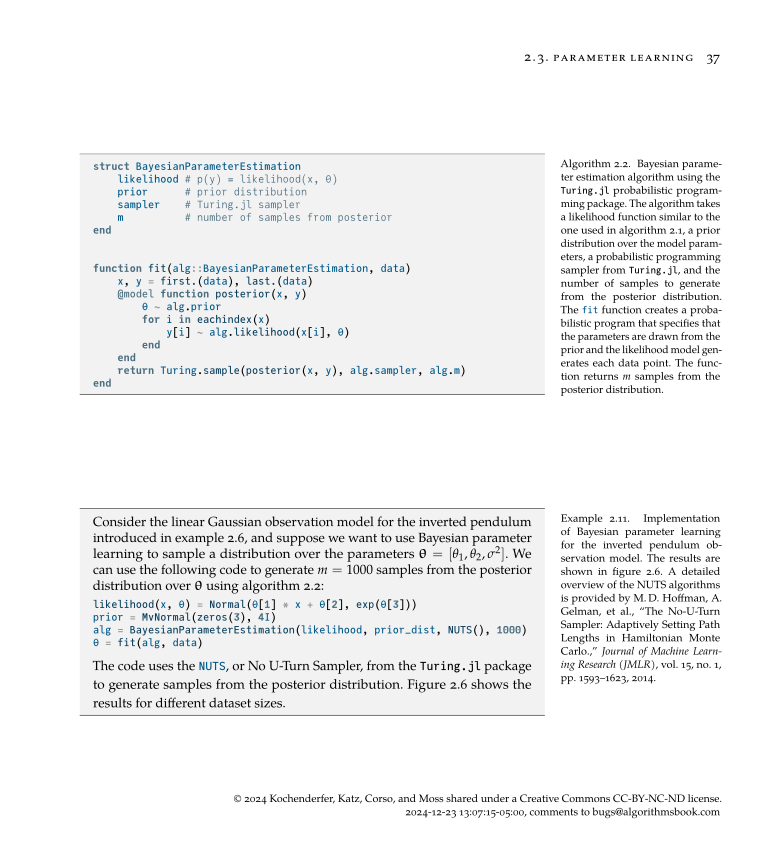
SELECT THE PARAMETERS FOR THE MODEL CLASS
Same sensor data, but now we learn a distribution over θ for N(o∣θ1s+θ2, θ32)
Data points used: {{ npTxt }}
p(θ1∣D)
E[θ1]= {{ bE0 }}
p(θ2∣D)
E[θ2]= {{ bE1 }}
p(θ3∣D)
E[θ3]= {{ bE2 }}
maximum likelihood
data used
models sampled from the posterior
SELECT THE PARAMETERS FOR THE MODEL CLASS
Sometimes, it is possible to compute the posterior analytically.
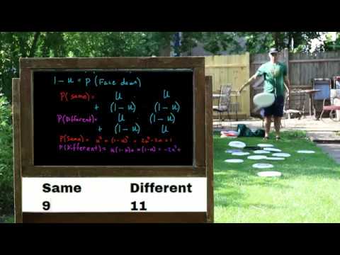
SELECT THE PARAMETERS FOR THE MODEL CLASS
Let’s flip frisbees!
SELECT THE PARAMETERS FOR THE MODEL CLASS
Let’s flip frisbees!
θ: probability of both frisbees landing in the same direction
1−θ: probability of both frisbees landing in different directions
Flip 10 times…
D={s,d,s,s,d,d,d,s,d,s}
n: number of times same
m: total number of flips
p(D∣θ)=θn(1−θ)m−n
Turns out that if we select our prior distribution to be p(θ)=Beta(θ∣α,β)…
our posterior will be p(θ∣D)=Beta(θ∣α+n, β+m−n)
SELECT THE PARAMETERS FOR THE MODEL CLASS
Let’s flip frisbees!
θ: probability of same
n: number of times same
m: total number of flips
p(θ)=Beta(θ∣α,β)
p(θ∣D)=Beta(θ∣α+n, β+m−n)
Some Notes
I skipped over the actual calculation of the posterior using this equation:
p(θ∣D)=∫θp(D∣θ)p(θ)dθp(D∣θ)p(θ)
You can either trust me or check out Chapter 4 of Algorithms for Decision Making.
The Beta distribution is a conjugate prior for the Bernoulli distribution: the posterior is in the same class as the prior.
See the demo for some intuition!
SELECT THE PARAMETERS FOR THE MODEL CLASS
Let’s flip frisbees!
Number same
{{ ns }}
Number different
{{ nd }}
Probability same is more likely: {{ pSame }}
SELECT THE PARAMETERS FOR THE MODEL CLASS
Many common distributions have conjugate priors
likelihood
conjugate prior
Bernoulli / binomial
Beta
multinomial
Dirichlet
Gaussian
Gaussian
SELECT THE PARAMETERS FOR THE MODEL CLASS
Many common distributions have conjugate priors
likelihood
conjugate prior
Bernoulli / binomial
Beta
multinomial
Dirichlet
Gaussian
Gaussian

likelihood model
conjugate prior
SELECT THE PARAMETERS FOR THE MODEL CLASS
What if we do have to make a choice though? 😬
SELECT THE PARAMETERS FOR THE MODEL CLASS
What if we do have to make a choice though? 😬
We can use the expectation of the distribution.
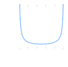
Although that might not be the best plan if the distribution is multimodal…
We can instead use the maximum a posteriori (MAP) estimate:
θ^=argmaxθP(θ∣D)
*sometimes also called the mode
SELECT THE PARAMETERS FOR THE MODEL CLASS
Two ways to learn θ from data
Point estimate
Maximum Likelihood
Pick the single θ that makes the data most likely
θ^=argmaxθ∑i=1mlogP(oi∣θ)
Output: one value θ̂
Distribution
Bayesian
Keep a belief over every possible θ
P(θ∣D)=∫θP(D∣θ)P(θ)dθP(D∣θ)P(θ)
Need one value? Use the expectation or MAP
SELECT THE PARAMETERS FOR THE MODEL CLASS
One last thing on parameter learning: we should be careful about generalization.
SELECT THE PARAMETERS FOR THE MODEL CLASS
One last thing on parameter learning: we should be careful about generalization.
We should evaluate our model on a separate validation set to make sure we are not overfitting.
Training Set
Validation Set
SELECT THE PARAMETERS FOR THE MODEL CLASS
One last thing on parameter learning: we should be careful about generalization.
We should evaluate our model on a separate validation set to make sure we are not overfitting.
Training Set
Validation Set
Holdout Method
K-fold Cross Validation
Plan for Today
1
General Thoughts on Models
2
Steps for Building Models
A
Select a Model Class
B
Select the Parameters for the Model Class
C
Validate the Model
VALIDATE THE MODEL
There is a story that has been going around about a physicist, a chemist, and an economist who were stranded on a desert island with only a can of food. The physicist and the chemist each devised an ingenious mechanism for getting the can open; the economist merely said, "Assume we have a can opener"!
VALIDATE THE MODEL
Our assumptions don’t mean much if they aren’t grounded in reality.
VALIDATE THE MODEL
Our assumptions don’t mean much if they aren’t grounded in reality.
All of our downstream validation results depend on how good our model is!
VALIDATE THE MODEL
Our assumptions don’t mean much if they aren’t grounded in reality.
All of our downstream validation results depend on how good our model is!
So we need to validate the model.
VALIDATE THE MODEL
We want to compare features of the model to features of the data.
VALIDATE THE MODEL
We want to compare features of the model to features of the data.
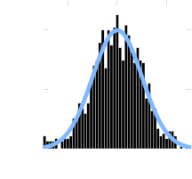
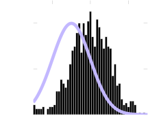
PDF Plot
good fit
bad fit
VALIDATE THE MODEL
We want to compare features of the model to features of the data.
good fit
bad fit
PDF Plot
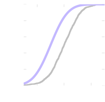
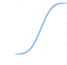
CDF Plot
VALIDATE THE MODEL
We want to compare features of the model to features of the data.
PDF Plot
good fit
bad fit
CDF Plot
VALIDATE THE MODEL
We want to compare features of the model to features of the data.
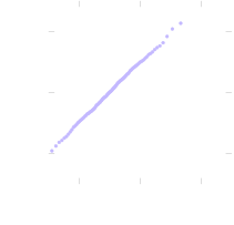
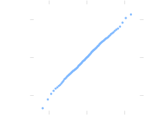
Quantile-Quantile (Q-Q) Plot
PDF Plot

α=0.1
qmodel=−2.28
qdata=−1.29
VALIDATE THE MODEL
We want to compare features of the model to features of the data.
Quantile-Quantile (Q-Q) Plot
PDF Plot
α=0.1
qmodel=−2.28
qdata=−1.29

VALIDATE THE MODEL
We want to compare features of the model to features of the data.
Quantile-Quantile (Q-Q) Plot
PDF Plot
VALIDATE THE MODEL
We want to compare features of the model to features of the data.
Quantile-Quantile (Q-Q) Plot
PDF Plot
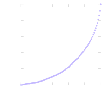
Calibration Plot
VALIDATE THE MODEL
We want to compare features of the model to features of the data.
Quantile-Quantile (Q-Q) Plot
PDF Plot
Calibration Plot
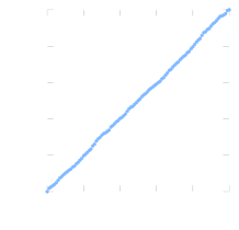
CDF Plot
good fit
bad fit
VALIDATE THE MODEL
We want to compare features of the model to features of the data.
Quantile-Quantile (Q-Q) Plot
PDF Plot
Calibration Plot
CDF Plot
good fit
bad fit
These are visual diagnostics. We can summarize them using summary metrics.
VALIDATE THE MODEL
PDF Plot
good fit
bad fit
These are visual diagnostics. We can summarize them using summary metrics.
We can summarize the PDF plot using the Kullback-Leibler divergence (K-L divergence).
DKL(p∥q)=∫p(x)log(q(x)p(x))dx
DKL=8.6×10⁻⁵
DKL=0.49
The K-L divergence is part of a broad class of divergences called the F-divergences.
The K-L divergence is not symmetric and it is not defined if the support of p is not a subset of the support of q.
The K-L divergence is not symmetric and it is not defined if the support of p is not a subset of the support of q.
VALIDATE THE MODEL
good fit
bad fit
These are visual diagnostics. We can summarize them using summary metrics.
We can summarize the CDF plot using the Kolmogorov-Smirnov statistic (K-S statistic).
CDF Plot
DKS=maxx∣P(X≤x)−Q(X≤x)∣
VALIDATE THE MODEL
good fit
bad fit
These are visual diagnostics. We can summarize them using summary metrics.
We can summarize the calibration plot using the Maximum Calibration Error (MCE) and Expected Calibration Error (ECE).
Calibration Plot
Average Gap
VALIDATE THE MODEL
What if we want to compare multiple features?
We need to be careful!
We don’t want to miss the interactions between features.

VALIDATE THE MODEL
We don’t want to miss the interactions between features.
One option: create a single feature that captures the relationship between multiple features.
VALIDATE THE MODEL
We don’t want to miss the interactions between features.
One option: create a single feature that captures the relationship between multiple features.
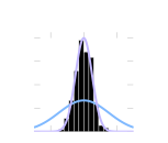
Multiple Features
Combined Feature
Multiple Features
VALIDATE THE MODEL
We don’t want to miss the interactions between features.
One option: create a single feature that captures the relationship between multiple features.
Combined Feature
Another option: extend summary metrics to multiple dimensions.
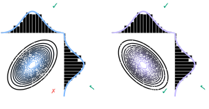
VALIDATE THE MODEL
What about conditional distributions?
Combined Feature
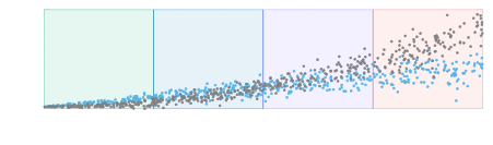
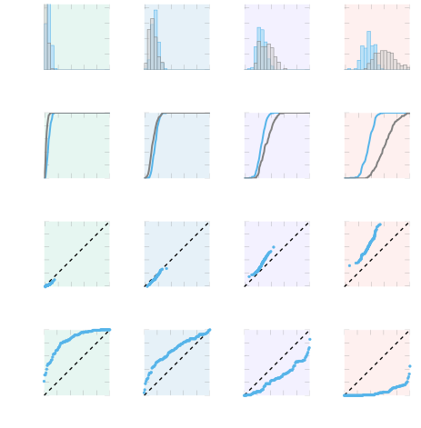
Partition conditioning variable into bins and compute visual diagnostics and metrics for each bin.
VALIDATE THE MODEL
Combined Feature
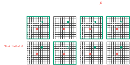
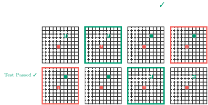
We can also validate models using expert knowledge.
VALIDATE THE MODEL
Combined Feature
We can also validate models using expert knowledge.
VALIDATE THE MODEL
Combined Feature
We can also validate models using expert knowledge.
Plan for Today
1
General Thoughts on Models
2
Steps for Building Models
A
Select a Model Class
B
Select the Parameters for the Model Class
C
Validate the Model